Excel syntax for CHOOSE(): |
|---|
=CHOOSE(index_num, value1[, value2][, value3][, …]) |
Excel syntax for MATCH(): |
|---|
=MATCH(lookup_value, lookup_array, [match_type]) |
| Syntax for CHOOSE-MATCH: |
|---|
=CHOOSE(MATCH(lookup_value, lookup_array, [match_type]), value1, [value2][, value3][, …]) |
Unlike the rewrite using VLOOKUP(), this rewrite uses one function as input for another function. MATCH() is nested inside CHOOSE(). CAD in D5 will use CHOOSE-MATCH.
Referring to the tables at the top of this post, these are the values needed by MATCH() in cell D5:
MATCH() item | Cell(s) or range | Value | Comments |
|---|---|---|---|
lookup_value | B5 | CAD | Given in the Foreign Currencies table |
lookup_array | $G$3:$G$10 | AUD..ZAR | Column 1 of the Exchange Rates table |
match_type | N/A * | FALSE | Similar to range_lookup in VLOOKUP() |
The dirty work will be done by MATCH(). Once it finds the position of CAD in lookup_array, it will feed it to the index_num used by CHOOSE(). CAD is listed in 2nd place in lookup_array.
The MATCH() used in D5 should look like this:
| // FALSE and 0 are equivalent; it’s used here for clarity. |
|---|
=MATCH(B5, $G$3:$G$10, FALSE) |
Again referring to the tables, these are the values needed by CHOOSE() in D6:
CHOOSE() item | Cell(s) or range | Value | Comments |
|---|---|---|---|
index_num | See Comments | See Comments | Result from MATCH() is fed to index_num |
value1 | $H$3 | 0.771950 | Required– a list needs at least 1 item |
value2 | $H$4 | 0.785590 | Optional– include as needed |
| TBD | ▬▬▬▬▬► | Note: ▬► | These 8 values are taken from Column 2 of the Exchange Rates table. |
value8 | $H$10 | 0.066029 | See Note above |
CHOOSE() looks like a complicated function, but it really requires 2 things: an index_num and a list of 1 value or more (and usually it’s more). Whatever value index_num has is the position of the value to take from the variable list of values. In this case, index_num turns out to be 2.
Replace index_num from CHOOSE() below with the MATCH() from above:
| The complete CHOOSE-MATCH formula: |
|---|
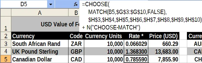
=CHOOSE(MATCH(B5, $G$3:$G$10, FALSE), $H$3, $H$4, $H$5, $H$6, $H$7, $H$8, $H$9, $H$10) |
Note that MATCH() finds the position of B5 (CAD) within Column 1 of the Rate table before it looks for its corresponding Rate in Column 2 (0.785590). Those rates are used in the value list of CHOOSE().
Why was MATCH() used in the first place? CAD may be 2nd in the list of 8 currencies, but what if additional currencies are added to the list and the list is resorted? CAD falls down the list, and who knows where that position is then? To avoid headaches at a later date, using MATCH() here makes CHOOSE-MATCH more useful.
This excerpt is taken from 8 Ways To Rewrite Nested IF() Functions at Magna Carta XLS Communications. Each of the 8 nested IF() rewrites from that post will be featured in its own post here.
Other posts will be migrated to this blog before I begin writing posts natively here.