Excel syntax for VLOOKUP(): |
|---|
=VLOOKUP(lookup_value, table_array, col_index_num, [range_lookup]) |
Excel syntax for CHOOSE(): |
|---|
=CHOOSE(index_num, value1[, value2][, value3][, …]) |
| Syntax for VLOOKUP-CHOOSE |
|---|
=VLOOKUP(lookup_value, CHOOSE(index_num, value1[, value2][, value3][, …]), col_index_num, [range_lookup]) |
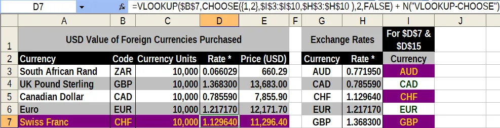
CHF– the Swiss Franc– will be used in D7 to show how VLOOKUP-CHOOSE works to rewrite nested IF()s.
Rewrite #1 for VLOOKUP() showed how convenient VLOOKUP() is compared to the nested IF()s it replaces. However, Rewrite #3 for INDEX-MATCH also noted that VLOOKUP() has a limitation:
VLOOKUP() cannot lookup values in columns to the left of lookup_value . |
|---|
When VLOOKUP() is used as written, that is true.
The limitation appears to be caused by table_array, since that determines how the lookup is to take place.
What if table_array can be redefined to be able to let VLOOKUP() look left?
CHOOSE() is used here to redefine table_array so that it can look left while it behaves as if it looks right.
As a reminder, this is how CHOOSE() is normally used:
=CHOOSE(index_num, value1[, value2][, value3][, …]) |
|---|
Below are the modifications to make to CHOOSE() before it can be used by VLOOKUP() to look left:
CHOOSE() item | Normal Data | Modification for VLOOKUP() |
|---|---|---|
index_num | Single cell or value | array of 2 values |
value1 | Single cell or value | range or column reference |
value2 | Single cell or value | range or column reference |
Based on those modifications, this is the revised syntax for VLOOKUP-CHOOSE:
| REVISED syntax for VLOOKUP-CHOOSE |
|---|
=VLOOKUP(lookup_value, CHOOSE({1,2[, …]}, desired_column1, desired_column2[, …]), col_index_num, [range_lookup]) |
For purposes of showing VLOOKUP-CHOOSE in action, a 3rd column was added to the Exchange Rates table. This 3rd column is just a duplicate of Column 1. This means the rates to be found in Column 2 are located to the left Column 3.
The index_num of CHOOSE() to be used here is an array of 2 numbers (1 followed by 2). After this array are the ranges or columns to be presented for use by CHOOSE() to VLOOKUP().
The first range or column to be listed in CHOOSE()— regardless of its order on the screen– will be assigned 1 from the array defining index_num. The second range or column will be assigned 2. When VLOOKUP() goes to table_array to use the column designated by CHOOSE(), it will choose the range or column mapped to the number 1.
VLOOKUP-CHOOSE for finding the rate for CHF (the Swiss Franc) should look like this:
=VLOOKUP(B7, CHOOSE({1,2}, $I$3:$I$10, $H$3:$H$10), 2, FALSE) |
|---|
| Note: |
|---|
For Excel 2010 and later, entire columns can be referenced, so for those versions CHOOSE({1,2},$I:$I,$H:$H) would be OK. I used Excel 2003, so it was necessary to use actual ranges limited to cells in the table. |
This excerpt is taken from 8 Ways To Rewrite Nested IF() Functions at Magna Carta XLS Communications. Each of the 8 nested IF() rewrites from that post will be featured in its own post here.
Other posts will be migrated to this blog before I begin writing posts natively here.